6 Ways to Optimize BigQuery Queries (and Save Time & Money)

BigQuery is powerful — but it can also be expensive and slow if you don’t know what you’re doing. It's easy to accidentally scan terabytes of data when you only meant to query a few gigabytes. Mistakes like these can end up costing hundreds (and sometimes thousands) of dollars.

In this post, we'll walk through six practical things that you can do to optimize your SQL queries and avoid a surprise BigQuery bill at the end of the month.

1. Leverage Partition Keys

Partitioning involves breaking down a large table into smaller segments based on the values in a specific column, which we call the "partition key". When you query a table and filter by partition key, BigQuery skips or "prunes" partitions that don't contain relevant data based on your filter conditions. This can significantly improve query performance and reduce costs by allowing BigQuery to scan only the relevant partitions.

Let's say we want to query web session data. The original table has 10 years worth of data but we only care about the past 3 months. We can write our query with a partition filter to reduce the amount of data that gets scanned:

SELECT count(*) AS n_sessions
FROM web_session_data
WHERE session_date >= DATE_SUB(CURRENT_DATE, INTERVAL 3 MONTH)

In the BigQuery console, you can tell if a table is partitioned based on the little symbol beside the table name. Partitioned tables have a symbol that looks like a table cut in half:

You can view the partition configs (e.g., partition key, partition granularity, and whether a partition filter is required) under the "Details" tab in the console:

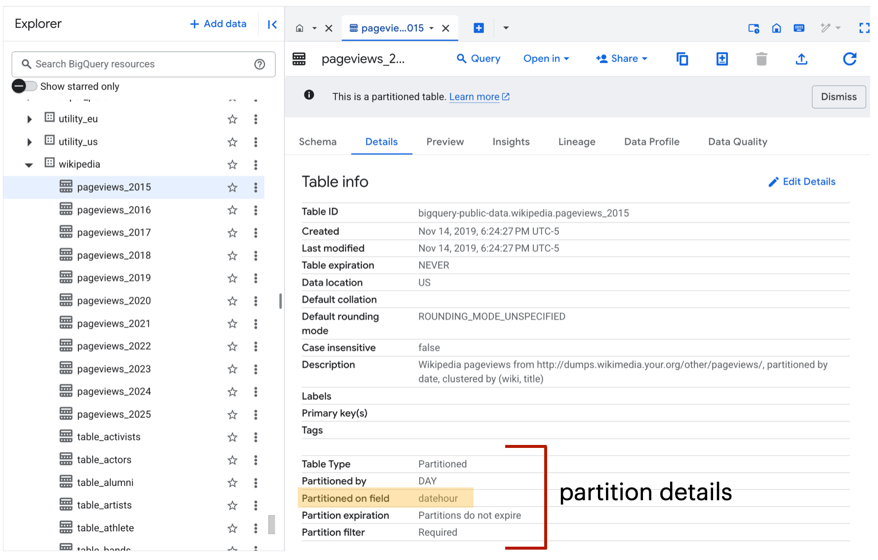
In most cases, a table's partition key will either be a date or datetime column. Time-based partitioning is especially common for temporal data like logs, events, and transactions. In rare cases, a partition key can be a categorical variable like country code or customer ID.

In the example above, we can see that a partition filter is required. This means that if you query the table without using a partition filter, the query will fail:

SELECT count(*) AS n_pageviews
FROM `bigquery-public-data.wikipedia.pageviews_2015` 

returns:

You'll have to update your query like this in order for it work:

SELECT count(*) AS n_pageviews
FROM `bigquery-public-data.wikipedia.pageviews_2015` 
WHERE TIMESTAMP_TRUNC(datehour, DAY) = TIMESTAMP("2015-09-01") 

returns 150363219. Success!!! ✅ With partition filtering, we're reducing the bytes processed, which directly lowers runtime and cost. It's a win-win situation.

2. Use Approximate Aggregations

Sometimes, exact numbers aren’t worth the cost. BigQuery charges based on bytes scanned, and operations like counting distinct users or calculating precise medians can be slow and expensive at scale. That’s where approximate aggregation functions come in. These functions use statistical algorithms to return results that are "good enough" for most analytics use cases (often with 99% accuracy) while running much faster and cheaper.

Let's say we run a social media platform and want to know how many unique users have signed up with us. We can query our entire table of users like this:

SELECT count(distinct user_id)
FROM all_users

This query looks innocent but because all_users is a massive table with millions of rows, it's going to be slow to run and very expensive. If you can tolerate an answer that's close enough, you should use the APPROX_COUNT_DISTINCT function instead:

SELECT APPROX_COUNT_DISTINCT(user_id)
FROM all_users

This simple change can reduce your query execution time from minutes to seconds at a fraction of the cost.

Approximate functions are great but they're not ideal for every situation. If you’re doing financial reporting or conducting an audit where every single record must be accounted for exactly, it's better to stick with the precise functions even if they’re slower and more expensive. But for the majority of data science workflows, approximate aggregations are a practical way to keep your queries fast and cost-effective.

3. Tread Carefully with CTEs

A common table expression (also known as CTE) is a temporary, named subquery that helps organize complex SQL logic into smaller, more digestible pieces.

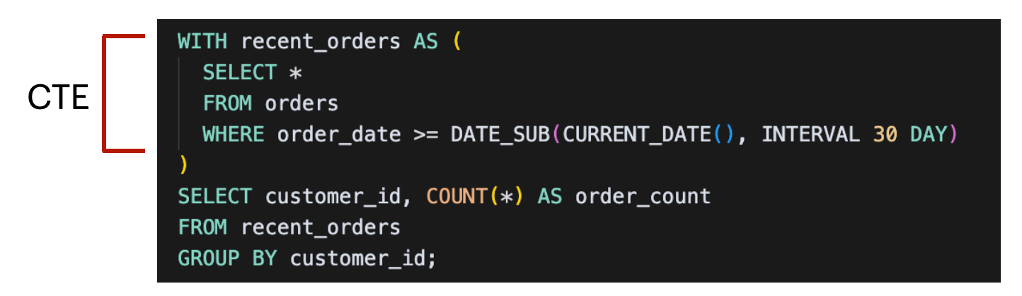
In some databases, CTEs are optimized and cached automatically, so if you reference the same CTE multiple times, it’s only executed once. BigQuery works differently. Each time you reference a CTE, BigQuery may re-run it in full, scanning the same data repeatedly. This can lead to higher costs and slower performance — especially if the CTE contains expensive operations like joins or large table scans.

The key to using CTEs effectively in BigQuery is to prioritize readability first, then optimize once you understand how BigQuery is executing your query. CTEs are fantastic for making your SQL easier to maintain, but be cautious about repeating expensive ones. If you need to reuse the same heavy logic multiple times, consider saving the results to a temporary table or creating a materialized view instead.

If you’re not sure whether a CTE is being scanned more than once, you don’t have to guess. You can use BigQuery's query execution plan to see how your query runs and where the most expensive steps are happening. Let's dig into this a bit more in Tip #4!

4. Use the Query Execution Plan

Once you’ve written a query, it’s not always obvious why it’s slow or expensive — especially if you’re working with multiple joins, nested subqueries, or large datasets. With BigQuery’s query execution plan, you can see exactly how your query runs behind the scenes.

Let's say we have a query that counts the distinct number of cabs at a given pickup/drop-off area in Chicago:

SELECT
  pickup_community_area,
  dropoff_community_area,
  APPROX_COUNT_DISTINCT(taxi_id) AS approx_unique_cabs
FROM `bigquery-public-data.chicago_taxi_trips.taxi_trips`
WHERE DATE_TRUNC(DATE(trip_start_timestamp), MONTH) = DATE '2016-02-01'
GROUP BY ALL
ORDER BY approx_unique_cabs DESC;

After running the query, we can inspect each stage of the execution plan, along with how many data was processed, how long it took, and whether any data shuffling occurred. This information is available under the "Execution Graph" and "Execution Details" tabs in the BigQuery console:

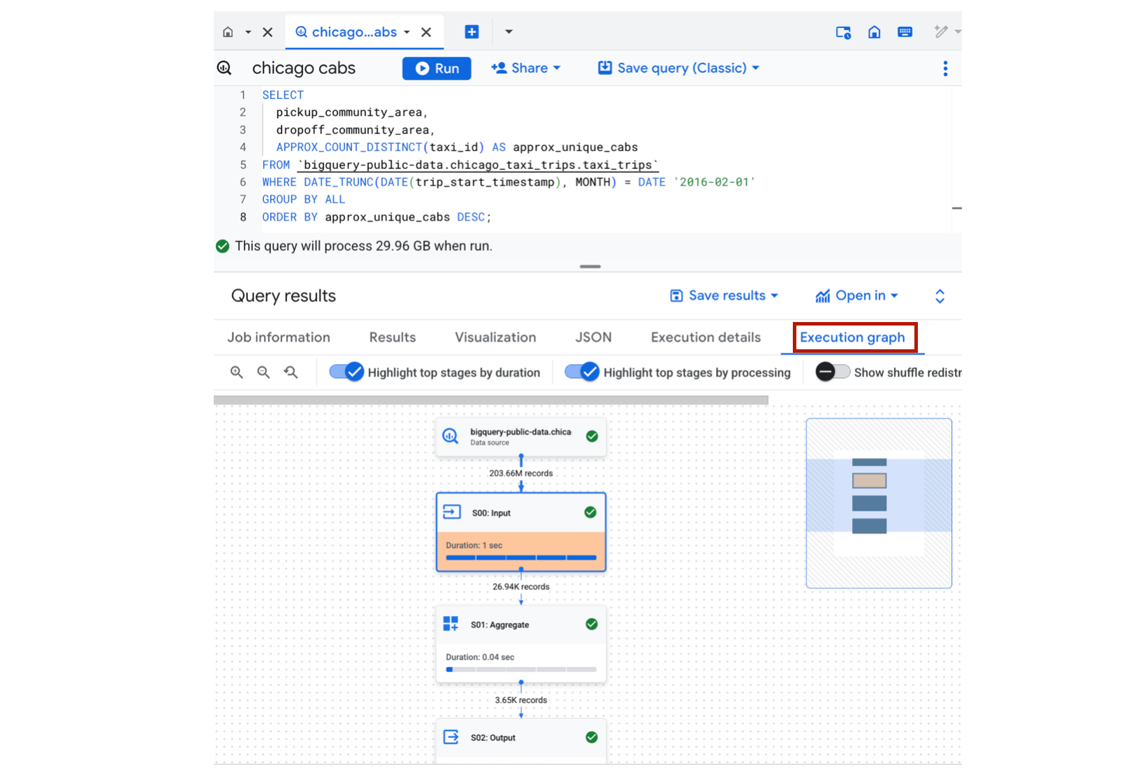
In this particular query plan, we can see that only Feb 2016 data is being scanned, and we're leveraging BigQuery's HyperLogLog algorithm to approximate a distinct count of taxi cabs. Pretty cool!!

Note that the query execution plan is only available after running the query. So this is more useful for situations where you want to run a query multiple times (i.e., on a schedule).

5. Take Advantage of Column Pruning

BigQuery supports column pruning which means that it will only scan the columns that you reference in a query. To understand why this works, it helps to know that BigQuery is a column-oriented database. This means that data is stored by column instead of by row like in MySQL and Postgres.

Columnar data storage is incredibly efficient for analytics. Let's say you want to query a very wide table with 200 columns but you only care about 5 of those columns. If you explicitly select 5 columns in your query, BigQuery will read just those 5 columns and ignore the other 195 columns. This translates directly into less data scanned, lower query costs, and faster performance. Clearly, a winning situation. 🙌

6. Use the Preview Feature to Inspect a Table

When you're exploring a table, it's very tempting to run a simple query like:

SELECT *
FROM new_table
LIMIT 5

While this query might look innocent, it can end up being very costly if the table in question (in this case, new_table) is terabytes in size. As discussed in an earlier BigQuery post,  this is because BigQuery is scanning every column in every row - even if you're limiting the output to 5 rows. If the goal of your query is to familiarize yourself with a table, you should consider using the Preview feature in the BigQuery console.

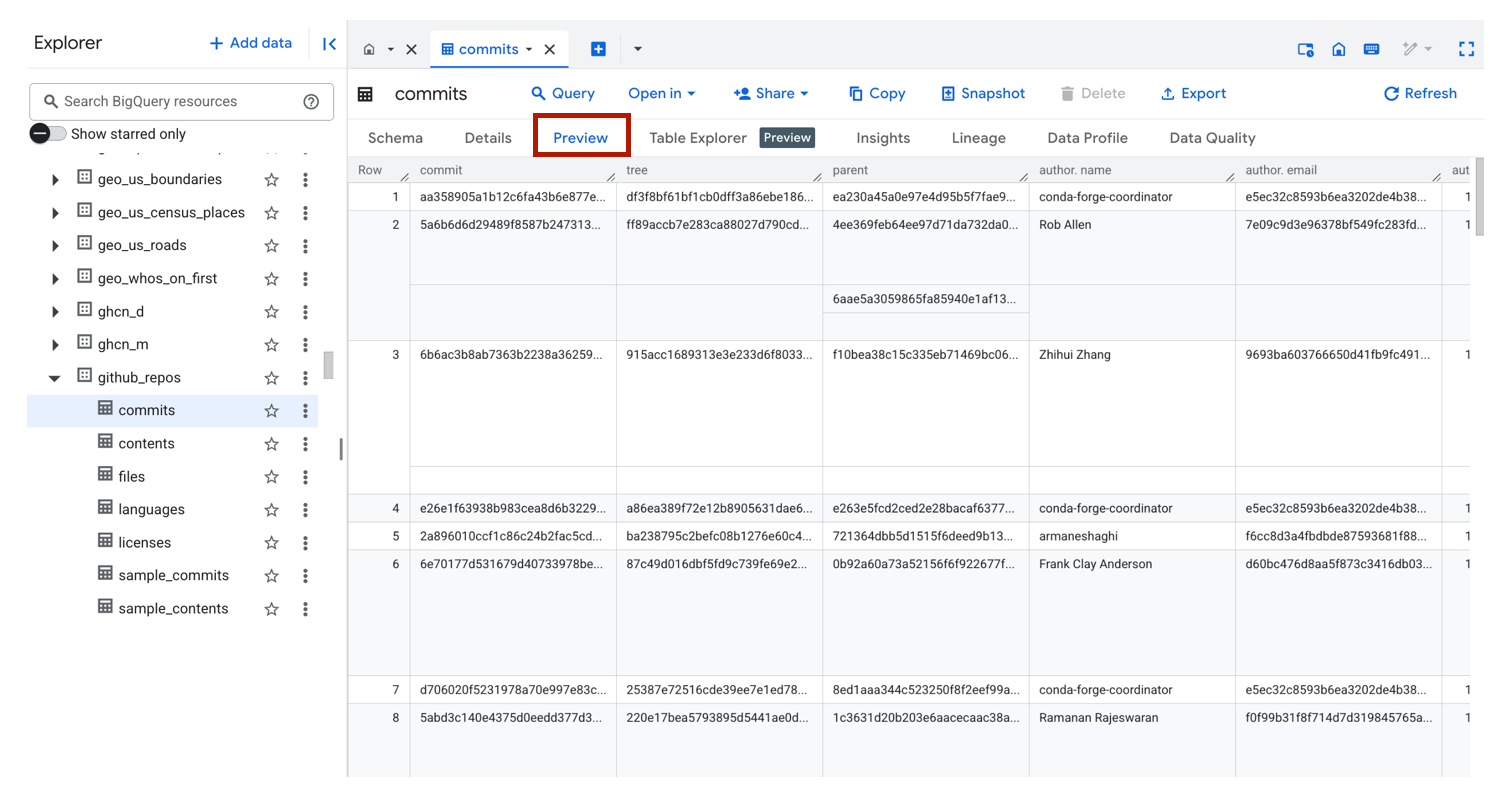
Under the Preview tab, you will get a glimpse of your table without actually scanning any data. I'll take a freebie any day.

Wrapping Up

BigQuery makes working with massive datasets easy, but it’s also easy to run up costs if you’re not careful. By leveraging partitioning, approximate aggregations, column pruning, and other optimization techniques, you can dramatically reduce both query time and costs — all while keeping your workflows efficient and scalable.

If you’ve got a performance optimization trick that I didn’t cover here, please share in the comments! Until next time ✌️