5 BigQuery Features Every Data Scientist Should Know

I use BigQuery almost every day at work and have grown to love it over the years. The learning curve was steep at first — from understanding how queries are billed to syntax differences (I was using Trino/Presto previously) to figuring out performance best practices. But once I got the hang of things, I came to really appreciate BigQuery and all of its amazing features.

Here are five BigQuery features that I think every data scientist should know.

1. Don’t Use SELECT * — Use Preview or TABLESAMPLE Instead

Let's say you want to inspect a new table. You might be tempted to run a query like:

SELECT *
FROM table_name
LIMIT 10;

This seems harmless – you're only querying 10 rows, right?!

Behind the scenes, BigQuery scans all referenced columns when you use SELECT *, it scans every column in every row - even if you're limiting the output to a handful of rows. This can end up costing a lot, especially when you're working with very wide tables.

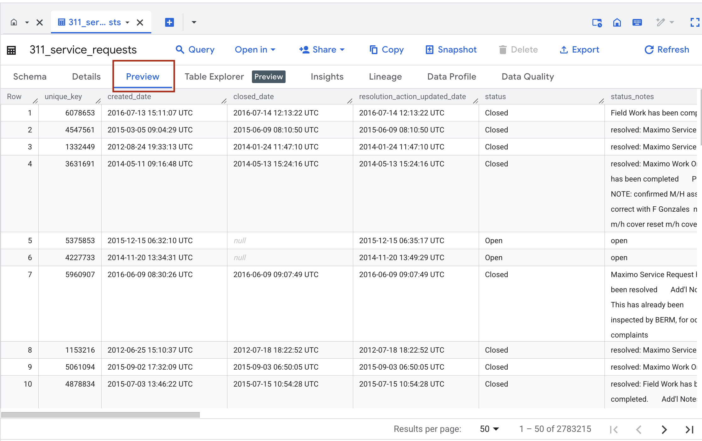
To avoid an unexpected bill in BigQuery, I recommend using the Preview tab in the console. It lets you see a sample of your table without actually scanning any data.

If you don’t want to use the Preview feature and prefer running a query, I highly recommend using BigQuery's TABLESAMPLE function. TABLESAMPLE lets you limit how much data gets scanned by randomly sampling subsets of data from the original table. You can specify the percentage of data you want to query like this:

SELECT *
FROM table_name
TABLESAMPLE SYSTEM (1 PERCENT)

In the query above, we're limiting the data to 1% of the entire table. This is a great feature for exploration and understanding unfamiliar datasets.

2. Use UDFs to Clean Up Your SQL

As a data scientist, your SQL queries can get messy — especially with repeated logic. To clean up your queries, you can write user-defined functions (also known as UDFs) which are reusable functions that you can apply directly in your SQL queries.

Let's say we want to clean up strings by removing special characters. You can create a UDF called remove_special_characters like this:

CREATE TEMP FUNCTION remove_special_characters(input STRING)
RETURNS STRING
AS (
  REGEXP_REPLACE(TRIM(input), r'[^a-zA-Z0-9 ]', '')
);

Now, you can easily use the remove_special_characters UDF in one of your queries:

SELECT 
  remove_special_characters(city_name) AS city_name,
  remove_special_characters(country_name) AS country_name
FROM sales

The beauty of UDFs is that they represent a single source of truth for your clean-up logic. If other teams are interested in using your UDF, you can publish it across your organization for other teammates to use.

3. Query External Data Using Federated Queries

Exploring data often means pulling from multiple systems. With BigQuery's federated queries, you can connect to external sources and run SQL over them instantly, without the overhead of loading new tables into BigQuery.

With federated queries, you can connect BigQuery directly to:

• Google Sheets
• CSV, JSON, Parquet files in Google Cloud Storage (GCS) or Google Drive
• And other cloud services like AWS S3 or Azure Blob Storage (!!!)

Let’s say we want to run a SQL query over a CSV file in Google Cloud Storage without importing it into BigQuery.

We first need to define the external table by assigning it a BQ dataset and table name, and provide the path of the CSV file:

CREATE EXTERNAL TABLE `your-project-id.analytics.raw_events_ext`
OPTIONS (
  format = 'CSV',
  uris = ['gs://my-bucket/path/to/files/*.csv'],
  autodetect = TRUE,
  field_delimiter = ',', 
  skip_leading_rows = 1,
  quote = '"',
  null_marker = '',
  max_bad_records = 0,
  encoding = 'UTF-8',
);

In the SQL snippet above, we're specifying some configs like the format of the external data source (in this case, CSV) and the delimiter (in this case, the comma). Since the CSV file has a header, we're skipping it by setting the skip_leading_rows argument to 1.

Once the external table is registered, we can query it like any other table in BigQuery. With federated queries, BigQuery is reading the CSV in place, which is pretty amazing. This means that if someone updates your CSV file, your queries will always reflect the latest values. Very cool!

4. Train Machine Learning Models in SQL with BigQuery ML

Did you know that you can train machine learning models in BigQuery using only SQL? With BigQuery ML, you can build regression models, classification models, time-series forecasting models and even deep neural networks directly in a SQL query. Here's an example of how we'd build a logistic regression model on a training dataset:

CREATE OR REPLACE MODEL `your-project-id.dataset.income_logreg`
OPTIONS (
  model_type = 'logistic_reg',
  input_label_cols = ['income_bracket']
) AS
SELECT
  age,
  hours_per_week,
  workclass,
  marital_status,
  occupation,
  relationship,
  race,
  sex,
  native_country,
  income_bracket
FROM `bigquery-public-data.ml_datasets.census_adult_income`
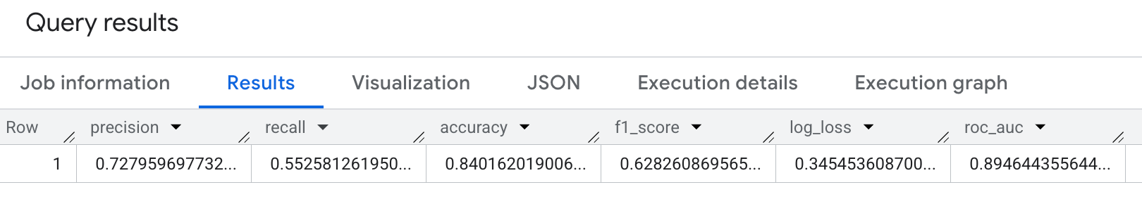
WHERE RAND() < 0.8;

Once the model above has been trained, you can evaluate it, run predictions, and even export the model for deployment. Here's an example of how we'd evaluate the model above on a holdout dataset:

SELECT *
FROM ML.EVALUATE(
  MODEL `your-project-id.dataset.income_logreg`,
  (
    SELECT
      age,
      hours_per_week,
      workclass,
      marital_status,
      occupation,
     relationship,
     race,
     sex,
     native_country,
     income_bracket
    FROM `bigquery-public-data.ml_datasets.census_adult_income`
    WHERE RAND() >= 0.8
  )
);

5. Use GROUP BY ALL For Quick Aggregations

When writing aggregation queries in SQL, you usually have to repeat every column you want to group by. For example:

SELECT 
  country,
  device_type,
  COUNT(*) AS sessions
FROM analytics.sessions
GROUP BY country, device_type

As you add more dimensions, your GROUP BY clause gets longer and more error-prone. If the column names in your "group by" don't match what's being aggregated in the SELECT statement, you'll end up seeing an error like this:

To avoid the headache of listing all columns in a GROUP BY, BigQuery makes this easier with the GROUP BY ALL shortcut. It works by automatically identifying all non-aggregated columns in the SELECT list.

So the same query above becomes:

SELECT 
  country,
  device_type,
  COUNT(*) AS sessions
FROM analytics.sessions
GROUP BY ALL

This is super useful when you're exploring data and don't want to maintain a long "group by" list. It also helps avoid mistakes when adding and removing columns in the SELECT clause. That said, GROUP BY ALL is less explicit – some teams prefer being verbose with column lists in production queries.

And that’s it — five BigQuery features I think every data scientist should know. These BigQuery features make my day-to-day work easier — I hope they do the same for you. 🫶